The Data Science Bowl is an annual data science competition hosted by Kaggle. In this year’s edition the goal was to detect lung cancer based on CT scans of the chest from people diagnosed with cancer within a year.
To tackle this challenge, we formed a mixed team of machine learning savvy people of which none had specific knowledge about medical image analysis or cancer prediction. Hence, the competition was both a nobel challenge and a good learning experience for us.
The competition just finished and our team Deep Breath finished 9th! In this post, we explain our approach.
The Deep Breath team consists of Andreas Verleysen, Elias Vansteenkiste, Fréderic Godin, Ira Korshunova, Jonas Degrave, Lionel Pigou and Matthias Freiberger. We are all PhD students and postdocs at Ghent University.
Introduction
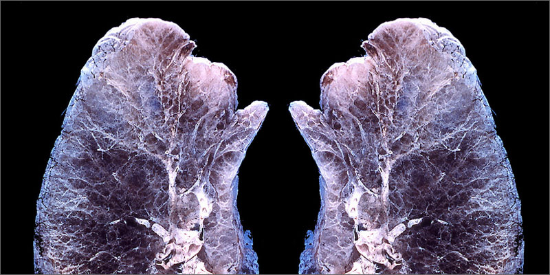
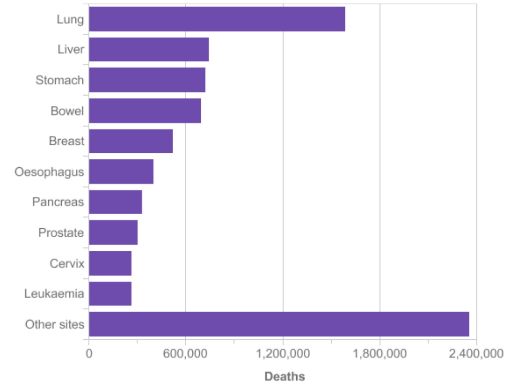
Lung cancer is the most common cause of cancer death worldwide. Second to breast cancer, it is also the most common form of cancer. To prevent lung cancer deaths, high risk individuals are being screened with low-dose CT scans, because early detection doubles the survival rate of lung cancer patients. Automatically identifying cancerous lesions in CT scans will save radiologists a lot of time. It will make diagnosing more affordable and hence will save many more lives.
To predict lung cancer starting from a CT scan of the chest, the overall strategy was to reduce the high dimensional CT scan to a few regions of interest. Starting from these regions of interest we tried to predict lung cancer. In what follows we will explain how we trained several networks to extract the region of interests and to make a final prediction starting from the regions of interest. This post is pretty long, so here is a clickable overview of different sections if you want to skip ahead:
- The Needle in The Haystack
- Nodule Detection
- False Positive Reduction
- Malignancy Prediction
- Lung Cancer Prediction
The Needle in The Haystack
To determine if someone will develop lung cancer, we have to look for early stages of malignant pulmonary nodules. Finding an early stage malignant nodule in the CT scan of a lung is like finding a needle in the haystack. To support this statement, let’s take a look at an example of a malignant nodule in the LIDC/IDRI data set from the LUng Node Analysis Grand Challenge. We used this dataset extensively in our approach, because it contains detailed annotations from radiologists. Given the wordiness of the official name, it is commonly referred as the LUNA dataset, which we will use in what follows.

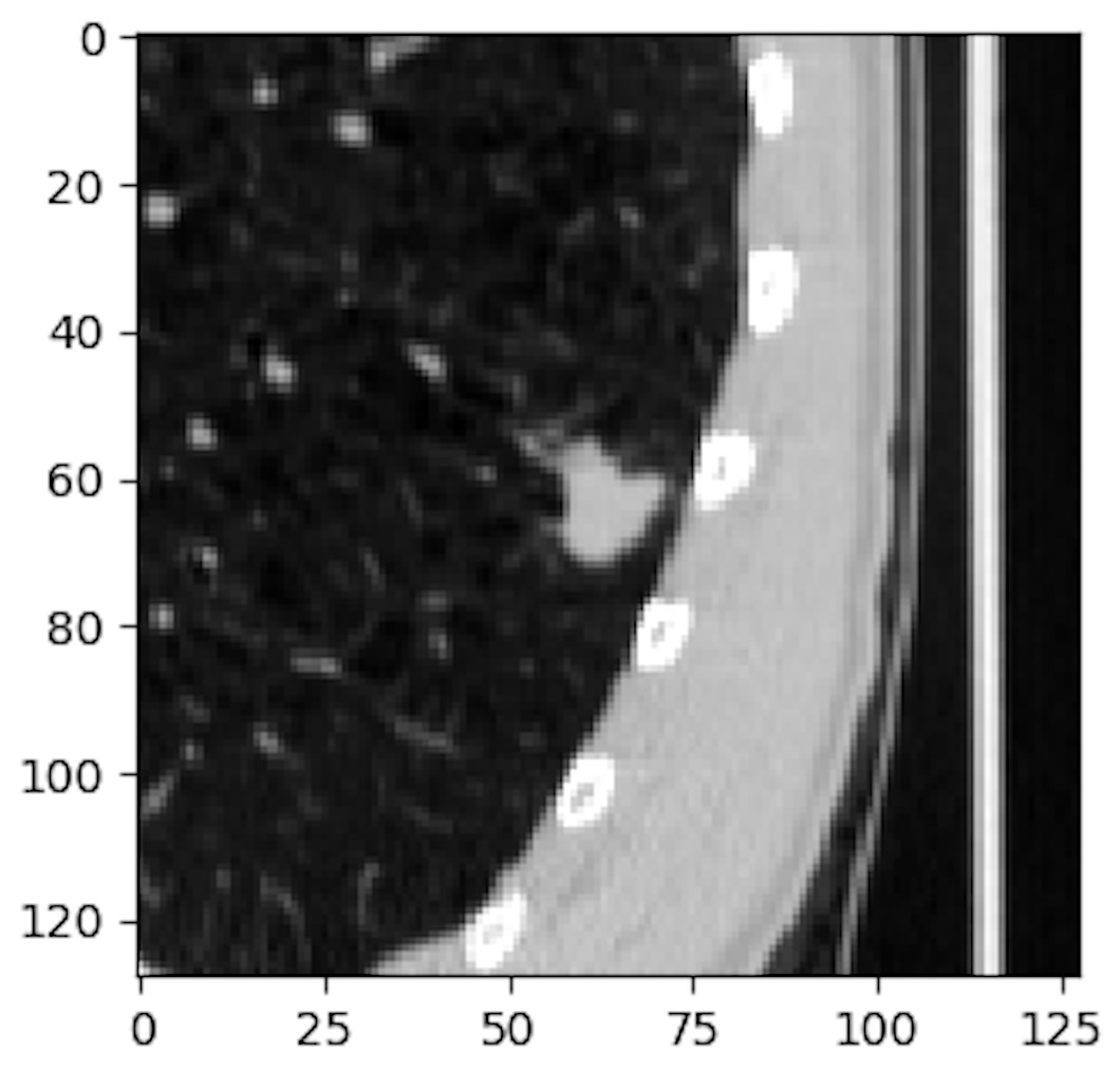

The radius of the average malicious nodule in the LUNA dataset is 4.8 mm and a typical CT scan captures a volume of 400mm x 400mm x 400mm. So we are looking for a feature that is almost a million times smaller than the input volume. Moreover, this feature determines the classification of the whole input volume. This makes analyzing CT scans an enormous burden for radiologists and a difficult task for conventional classification algorithms using convolutional networks.
This problem is even worse in our case because we have to try to predict lung cancer starting from a CT scan from a patient that will be diagnosed with lung cancer within one year of the date the scan was taken. TIn the LUNA dataset contains patients that are already diagnosed with lung cancer. In our case the patients may not yet have developed a malignant nodule. So it is reasonable to assume that training directly on the data and labels from the competition wouldn’t work, but we tried it anyway and observed that the network doesn’t learn more than the bias in the training data.
Nodule Detection
Nodule Segmentation
To reduce the amount of information in the scans, we first tried to detect pulmonary nodules. We built a network for segmenting the nodules in the input scan. The LUNA dataset contains annotations for each nodule in a patient. These annotations contain the location and diameter of the nodule. We used this information to train our segmentation network.
The chest scans are produced by a variety of CT scanners, this causes a difference in spacing between voxels of the original scan. We rescaled and interpolated all CT scans so that each voxel represents a 1x1x1 mm cube. To train the segmentation network, 64x64x64 patches are cut out of the CT scan and fed to the input of the segmentation network. For each patch, the ground truth is a 32x32x32 mm binary mask. Each voxel in the binary mask indicates if the voxel is inside the nodule. The masks are constructed by using the diameters in the nodule annotations.
intersection = sum(y_true * y_pred)
dice = (2. * intersection) / (sum(y_true) + sum(y_pred))
As objective function we choose to optimize the Dice coefficient. The dice coefficient is a commonly used metric for image segmentation. It behaves well for the imbalance that occurs when training on smaller nodules, which are important for early stage cancer detection. A small nodule has a high imbalance in the ground truth mask between the number of voxels in- and outside the nodule.
The downside of using the Dice coefficient is that it defaults to zero if there is no nodule inside the ground truth mask. There must be a nodule in each patch that we feed to the network. To introduce extra variation, we apply translation and rotation augmentation. The translation and rotation parameters are chosen so that a part of the nodule stays inside the 32x32x32 cube around the center of the 64x64x64 input patch.
The network architecture is shown in the following schematic. The architecture is largely based on the U-net architecture, which is a common architecture for 2D image segmentation. We adopted the concepts and applied them to 3D input tensors. Our architecture mainly consists of convolutional layers with 3x3x3 filter kernels without padding. Our architecture only has one max pooling layer, we tried more max pooling layers, but that didn’t help, maybe because the resolutions are smaller than in case of the U-net architecture. The input shape of our segmentation network is 64x64x64. For the U-net architecture the input tensors have a 572x572 shape.

The trained network is used to segment all the CT scans of the patients in the LUNA and DSB dataset. 64x64x64 patches are taken out the volume with a stride of 32x32x32 and the prediction maps are stitched together. In the resulting tensor, each value represents the predicted probability that the voxel is located inside a nodule.
Blob Detection
In this stage we have a prediction for each voxel inside the lung scan, but we want to find the centers of the nodules. The nodule centers are found by looking for blobs of high probability voxels. Once the blobs are found their center will be used as the center of nodule candidate.
In our approach blobs are detected using the Difference of Gaussian (DoG) method, which uses a less computational intensive approximation of the Laplacian operator. We used the implementation available in skimage package.
After the detection of the blobs, we end up with a list of nodule candidates with their centroids. Unfortunately the list contains a large amount of nodule candidates. For the CT scans in the DSB train dataset, the average number of candidates is 153. The number of candidates is reduced by two filter methods:
- Applying lung segmentation before blob detection
- Training a false positive reduction expert network
Lung Segmentation
Since the nodule segmentation network could not see a global context, it produced many false positives outside the lungs, which were picked up in the later stages. To alleviate this problem, we used a hand-engineered lung segmentation method.
At first, we used a similar strategy as proposed in the Kaggle Tutorial. It uses a number of morphological operations to segment the lungs. After visual inspection, we noticed that quality and computation time of the lung segmentations was too dependent on the size of the structuring elements. A second observation we made was that 2D segmentation only worked well on a regular slice of the lung. Whenever there were more than two cavities, it wasn’t clear anymore if that cavity was part of the lung.

Our final approach was a 3D approach which focused on cutting out the non-lung cavities from the convex hull built around the lungs.


False Positive Reduction
To further reduce the number of nodule candidates we trained an expert network to predict if the given candidate after blob detection is indeed a nodule. We used lists of false and positive nodule candidates to train our expert network. The LUNA grand challenge has a false positive reduction track which offers a list of false and true nodule candidates for each patient.
For training our false positive reduction expert we used 48x48x48 patches and applied full rotation augmentation and a little translation augmentation (±3 mm).
Architecture
If we want the network to detect both small nodules (diameter <= 3mm) and large nodules (diameter > 30 mm), the architecture should enable the network to train both features with a very narrow and a wide receptive field. The inception-resnet v2 architecture is very well suited for training features with different receptive fields. Our architecture is largely based on this architecture. We simplified the inception resnet v2 and applied its principles to tensors with 3 spatial dimensions. We distilled reusable flexible modules. These basic blocks were used to experiment with the number of layers, parameters and the size of the spatial dimensions in our network.

The first building block is the spatial reduction block. The spatial dimensions of the input tensor are halved by applying different reduction approaches. Max pooling on the one hand and strided convolutional layers on the other hand

The feature reduction block is a simple block in which a convolutional layer with 1x1x1 filter kernels is used to reduce the number of features. The number of filter kernels is the half of the number of input feature maps.

The residual convolutional block contains three different stacks of convolutional layers block, each with a different number of layers. The most shallow stack does not widen the receptive field because it only has one conv layer with 1x1x1 filters. The deepest stack however, widens the receptive field with 5x5x5. The feature maps of the different stacks are concatenated and reduced to match the number of input feature maps of the block. The reduced feature maps are added to the input maps. This allows the network to skip the residual block during training if it doesn’t deem it necessary to have more convolutional layers. Finally the ReLu nonlinearity is applied to the activations in the resulting tenor.
We experimented with these bulding blocks and found the following architecture to be the most performing for the false positive reduction task:
def build_model(l_in):
    l = conv3d(l_in, 64)

    l = spatial_red_block(l)
    l = res_conv_block(l)
    l = spatial_red_block(l)
    l = res_conv_block(l)
    l = spatial_red_block(l)
    l = res_conv_block(l)

    l = feat_red(l)
    l = res_conv_block(l)
    l = feat_red(l)

    l = dense(drop(l), 128)

    l_out = DenseLayer(l, num_units=1, nonlinearity=sigmoid)
    return l_out
An important difference with the original inception is that we only have one convolutional layer at the beginning of our network. In the original inception resnet v2 architecture there is a stem block to reduce the dimensions of the input image.
Results
Our validation subset of the LUNA dataset consists of the 118 patients that have 238 nodules in total. After segmentation and blob detection 229 of the 238 nodules are found, but we have around 17K false positives. To reduce the false positives the candidates are ranked following the prediction given by the false positive reduction network.
| Top | True Positives | False Positives |
|---|---|---|
| 10 | 221 | 959 |
| 4 | 187 | 285 |
| 2 | 147 | 89 |
| 1 | 99 | 19 |
Malignancy Prediction
It was only in the final 2 weeks of the competition that we discovered the existence of malignancy labels for the nodules in the LUNA dataset. These labels are part of the LIDC-IDRI dataset upon which LUNA is based. For the LIDC-IDRI, 4 radiologist scored nodules on a scale from 1 to 5 for different properties. The discussions on the Kaggle discussion board mainly focussed on the LUNA dataset but it was only when we trained a model to predict the malignancy of the individual nodules/patches that we were able to get close to the top scores on the LB.
def build_model(l_in):
    l = conv3d(l_in, 64)

    l = spatial_red_block(l)
    l = res_conv_block(l)
    l = spatial_red_block(l)
    l = res_conv_block(l)

    l = spatial_red_block(l)
    l = spatial_red_block(l)

    l = dense(drop(l), 512)

    l_out = DenseLayer(l, num_units=1, nonlinearity=sigmoid)
    return l_out
The network we used was very similar to the FPR network architecture. In short it has more spatial reduction blocks, more dense units in the penultimate layer and no feature reduction blocks.
We rescaled the malignancy labels so that they are represented between 0 and 1 to create a probability label. We constructed a training set by sampling an equal amount of candidate nodules that did not have a malignancy label in the LUNA dataset.
As objective function, we used the Mean Squared Error (MSE) loss which showed to work better than a binary cross-entropy objective function.
Lung Cancer Prediction
After we ranked the candidate nodules with the false positive reduction network and trained a malignancy prediction network, we are finally able to train a network for lung cancer prediction on the Kaggle dataset. Our strategy consisted of sending a set of n top ranked candidate nodules through the same subnetwork and combining the individual scores/predictions/activations in a final aggregation layer.
Transfer learning
After training a number of different architectures from scratch, we realized that we needed better ways of inferring good features. Although we reduced the full CT scan to a number of regions of interest, the number of patients is still low so the number of malignant nodules is still low. Therefore, we focussed on initializing the networks with pre-trained weights.
The transfer learning idea is quite popular in image classification tasks with RGB images where the majority of the transfer learning approaches use a network trained on the ImageNet dataset as the convolutional layers of their own network. Hence, good features are learned on a big dataset and are then reused (transferred) as part of another neural network/another classification task. However, for CT scans we did not have access to such a pretrained network so we needed to train one ourselves.
At first, we used the the fpr network which already gave some improvements. Subsequently, we trained a network to predict the size of the nodule because that was also part of the annotations in the LUNA dataset. In both cases, our main strategy was to reuse the convolutional layers but to randomly initialize the dense layers.
In the final weeks, we used the full malignancy network to start from and only added an aggregation layer on top of it. However, we retrained all layers anyway. Somehow logical, this was the best solution.
Aggregating Nodule Predictions
We tried several approaches to combine the malignancy predictions of the nodules. We highlight the 2 most successful aggregation strategies:
- P_patient_cancer = 1 - ∏ P_nodule_benign: The idea behind this aggregation is that the probability of having cancer is equal to 1 if all the nodules are benign. If one nodule is classified as malignant, P_patient_cancer will be one. The problem with this approach is that it doesn’t behave well when the malignancy prediction network is convinced one of the nodules is malignant. Once the network is correctly predicting that the network one of the nodules is malignant, the learning stops.
- Log Mean Exponent: The idea behind this aggregation strategy is that the cancer probability is determined by the most malignant/the least benign nodule. The LME aggregation works as the soft version of a max operator. As the name suggest, it exponential blows up the predictions of the individual nodule predictions, hence focussing on the largest(s) probability(s). Compared to a simple max function, this function also allows backpropagating through the networks of the other predictions.
Ensembling
Our ensemble merges the predictions of our 30 last stage models. Since Kaggle allowed two submissions, we used two ensembling methods:
- Defensive ensemble: Average the predictions using weights optimized on our internal validation set. The recurring theme we saw during this process was the high reduction of the number of models used in the ensemble. This is caused by the high similarity between the models. It turned out that for our final submission, only one model was selected.
- Aggressive ensemble: Cross-validation is used to select the high-scoring models that will be blended uniformly. The models used in this ensemble are trained on all the data, hence the name ‘aggressive ensemble’. We uniformly blend these ‘good’ models to avoid the risk of ending up with an ensemble with very few models because of the high pruning factor during weight optimization. It also reduces the impact of an overfitted model. Reoptimizing the ensemble per test patient by removing models that disagree strongly with the ensemble was not very effective because many models get pruned anyway during the optimization. Another approach to select final ensemble weights was to average the weights that were chosen during CV. This didn’t improve our performance. We also tried stacking the predictions using tree models but because of the lack of meta-features, it didn’t perform competitively and decreased the stability of the ensemble.
Final Thoughts
A big part of the challenge was to build the complete system. It consists of quite a number of steps and we did not have the time to completely finetune every part of it. So there is stil a lot of room for improvement. We would like to thank the competition organizers for a challenging task and the noble end.
Hacking the leaderboard
Before the competition started a clever way to deduce the ground truth labels of the leaderboard was posted. It uses the information you get from a the high precision score returned when submitting a prediction. As a result everyone could reverse engineer the ground truths of the leaderboard based on a limited amount of submissions.
Normally the leaderboard gives a real indication of how the other teams are doing, but now we were completely in the dark, and this negatively impacted our motivation. Kaggle could easily prevent this in the future by truncating the scores returned when submitting a set of predictions.
The Deep Breath Team
Andreas Verleysen @resivium
Elias Vansteenkiste @SaileNav
Fréderic Godin @frederic_godin
Ira Korshunova @iskorna
Jonas Degrave @317070
Lionel Pigou @lpigou
Matthias Freiberger @mfreib